欢迎访问《控制理论与应用》期刊网站！

带LCL滤波器的三相并网逆变器的鲁棒电流跟踪控制

doi: 10.7641/CTA.2025.50051

刘伟¹ ，吴本¹ ，孙伟杰¹ ，雪映² ，蔡逢煌³

1. 华南理工大学自动化科学与工程学院自主系统与网络控制教育部重点实验室, 广东广州 510641

2. 华南理工大学电力学院, 广东广州 510641

3. 福州大学电气工程与自动化学院, 福建福州 350108

详细信息

作者简介

刘伟教授,博士生导师,目前研究方向为非线性控制、多智能体系统协同控制、机器人、无人机和电力系统的建模和控制,E-mail: weiliu@scut.edu.cn;

吴本博士研究生,目前研究方向为输出调节、非线性控制、事件触发控制、多智能体系统,E-mail: aubenwu@mail.scut.edu.cn;

孙伟杰副教授,目前研究方向为非线性控制、自适应和学习算法、电子设备的控制,E-mail: auwjsun@scut.edu.cn;

雪映教授,博士生导师,目前研究方向为含高比例可再生能源电力系统的稳定分析与智能控制、高压直流输电、电力系统电磁暂态仿真以及智能配电网技术,E-mail: dryingxue@scut.edu.cn;

蔡逢煌教授,博士生导师,目前研究方向为电力电子和控制、故障诊断和嵌入式系统,E-mail: caifenghuang@fzu.edu.cn.

通信作者

孙伟杰，E-mail: auwjsun@scut.edu.cn;Tel.:+8620-87111289.

Robust current tracking control for three-phase grid-connected inverters with LCL filter

LIU Wei¹ ， WU Ben¹ ， SUN Wei-jie¹ ， XUE Ying² ， CAI Feng-huang³

1. Key Laboratory of Autonomous Systems and Networked Control of Ministry of Education, School of Automation Science and Engineering, South China University of Technology, Guangzhou Guangdong 510641 , China

2. School of Electric Power Engineering, South China University of Technology, Guangzhou Guangdong 510641 , China

3. College of Electrical Engineering and Automation, Fuzhou University, Fuzhou Fujian 350108 , China

Funds: Supported by the Fundamental Research Funds for the Central Universities (2024ZYGXZR047), the National Natural Science Foundation of China (62373156) and the Guangdong Basic and Applied Basic Research Foundation (2024A1515011736).

摘要

本文采用动态状态反馈控制方法研究在外界干扰下带LCL滤波器的三相并网逆变器的鲁棒电流跟踪控制问题. 首先, 本文构建内模用于学习并网逆变器在稳态下的状态和输入信息. 其次, 利用内模原理, 基于一些合适的坐标变换将跟踪控制问题转化为鲁棒镇定控制问题. 然后, 设计一种动态状态反馈控制律来处理这一鲁棒镇定问题, 从而得到三相并网逆变器的鲁棒电流跟踪控制问题的解. 该控制方法能够保证闭环系统的渐近稳定性. 最后, 通过几组仿真验证提出的控制方法的有效性, 并将其与前馈控制方法做对比, 以验证本文提出的方法对不确定参数的鲁棒性.

关键词

并网逆变器 / 内模原理 / 电流跟踪 / 干扰抑制 / 鲁棒控制

Abstract

This article investigates the robust current tracking control problem of three-phase grid-connected inverters with LCL filter under external disturbance by a dynamic state feedback control method. First, this paper constructs an internal model to learn the information of the states and input of the grid-connected inverter under steady state. Second, by utilizing the internal model principle, the paper turns the tracking control problem into the robust stabilization control problem based on some appropriate coordinate transformations. Then, The paper designs a dynamics state feedback control law to deal with this robust stabilization problem, and thus the solution of the robust current tracking control problem of three-phase grid-connected inverters can be obtained. This control method can ensure the asymptotic stability of the closedloop system. Finally, the paper illustrates the effectiveness of the proposed control approach through several groups of simulations, and compares it with the feedforward control method to verify the robustness of the proposed control method to uncertain parameters.

Keywords

grid-connected inverter / internal model principle / current tracking / disturbance suppression / robust control

1 Introduction 2 Inverter model and problem formulation 3 Controller design and stability analysis 4 Simulation verification 5 Conclusions

1 Introduction

With the rapid development and increasing employment of renewable energy, grid-connected inverters have gained more and more attention because of its reliability and flexibility ^[1]. As the key components of micro-grids and distributed generation systems, the grid-connected inverters play an important role in providing effective interfaces for renewable and sustainable distributed energy resources.

The grid-connected inverters should operate in a stable way that its output current injecting into the network is as similar as the desired sinusoidal signal, in viewpoint of magnitude, phase and frequency. As such, LCL filters are widely used in grid-connected inverter for its better ability of attenuating the switchingfrequency harmonics ^[2]. This is important for modern power electronics devices requiring high power quality. However, due to the inherent resonance of LCL filters, the inverter systems are subject to instability problem ^[3]. Thus, passive damping techniques from the viewpoint of circuit design have been investigated to reduce the undesired resonant oscillation. Different approaches have been proposed such as modifying reactive elements with different topologies ^[4], using optimization algorithms for filters parameter design ^[5] and using adaptive observer and event-triggered mechanism for control mechanism ^[6] and the references therein. As drawbacks, the passive damping methods increase the filter volume and power losses ^[7].

To avoid the drawbacks, one alternative solution is to employ the active damping techniques, consisting in modifications of the control diagram without extra losses. Various control methods have been routinely used to enhance the performance of grid-connected inverters which, in general, include the popular proportional integral (PI) control ^[8-9] and proportional resonant (PR) control ^[10-11]. In ^[8], based on feedback linearization technique, a PI controller has been designed by combining a disturbance observer. Unfortunately, a main demerit of the feedback linearization technique is that the exact knowledge of model parameters needs to be known. In ^[9], based on system feedback ratio matrix, a novel perspective of stability analysis has been proposed, which is more suitable for engineering because of its low computational complexity and high accuracy. For the PR controller in stationary reference frame, as stated in ^[10], it is almost an equivalent alternative to synchronous frame PI controllers. It removes the computational-intensive transformation from stationary frame to synchronous frame ^[11] . By choosing a infinite gain at the chosen resonant frequency, it can theoretically achieve zero steady-state error.

In order to effectively achieve the current tracking for grid-connected inverters, research effort has been put into developing some other advanced control strategies because of the great computing power available from modern digital signal processors. Model predictive control (MPC) is designed to minimize the tracking error by defining a cost function ^[12], and therefore, it offers a straightforward way to include required constraints and nonlinearities in the control law. Its applications in the power electronics field can be found in ^[12-14]. In ^[13], an observer-based control architecture was proposed to reduce the required sensors, eliminate measurement noise and reduce the influence of grid disturbance and parameter uncertainty. In ^[14], by using the state estimator, the disturbance observer and the cost function, a sensorless MPC protocol based on the grid-side current measurement was proposed for a gridconnected inverter with LCL filter, which can suppress the filter resonance frequency component and against the variation of grid impedance.

The aforementioned literature for the active damping controller design hardly take into account robustness to external disturbance and parameter uncertainty. Variations of inverter parameters and grid impedance would result in changes of resonance frequency such that the original fixed control gains may fail to give the satisfactory performance. To overcome this challenge, sliding mode control (SMC) has been studied in recent work ^[15-17]. SMC has the ability to reject parameters deviations and undesirable disturbances. In ^[17], a finite-time full-order sliding mode method was proposed to enhance the response speed and robustness of the inverter system. In addition to SMC,

H_{\infty}

control has also been applied to enhance robust performance for its optimal rejection of external disturbances ^[18-20] . Such a control philosophy usually leads to high controller gains, since it is designed in order to guarantee the satisfactory performance specifications even for the worst-case uncertainties and disturbances. In ^[18], a linear matrix inequality condition has been proposed to obtain a less conservative controller for the grid-connected inverter. By mixing

H_{2}

quality criteria, the study in ^[19] aims to find a tradeoff between control gain and performance. In ^[20], by utilizing

H_{\infty}

observer, a faulttolerant controller was presented to achieve accurate voltage tracking and current sharing for DC microgrids with disturbances.

This article formulates the current tracking control problem of grid-connected inverters under the grid voltage disturbance in the output regulation scheme. The aim of output regulation control (ORC) is to obtain a feedback controller such that the out of a controlled plant can achieve asymptotic tracking with the ability of disturbance rejection, and furthermore, the trajectory of the closed-loop system exists and is bounded ^[21]. As opposed to the inversion-based tracking control, ORC is designed without requiring differential information knowledge of output tracking error. Hence, ORC provides a more reliable tracking solution since noise in the measured output would not be amplified by differentiation. On the other hand, the tracking performance under the inversion-based scheme is vulnerable to the measurement noise in practice such that the controlled system would even corrupt.

It is worth mentioning that a general framework has been established in ^[21], where, by using the internal model resulting from an elegant concept of steady-state generator, the output regulation problem can be converted into a stabilization problem. Such a framework lends itself to a greater flexibility of using various stabilization techniques such that the trajectory tracking with external disturbances can be guaranteed under the un-certain parameter ^[22]. The main contributions are as follows.

1) The paper considers the grid voltage disturbance while designing the current tracking controller for the grid-connected inverters. Moreover, in contrast to the recent work ^[23-25] using feedback linearization technique and disturbance observer scheme, the output regulation scheme is employed such that the proposed controller allows the parameter uncertainty.

2) The design philosophy gives an explicit step-bystep procedure to determine the controller gains such that, for parameters within any compact subset, the control objective can be achieved. This facilitates the adjustment of controller gains in actual implementations. Steady-state performance with robustness against different parameter settings is remarkable, as verified by simulations.

3) The output regulation framework based on internal model principle proposed in ^[21] is first applied to grid-connected inverters. Under this framework, theparameter uncertainty and the grid-connected voltage disturbance can be handled and the current asymptotic tracking can be achieved simultaneously.

2 Inverter model and problem formulation

Fig.1 shows the control schematic diagram of the distributed generation (DG) interfacing system, which consists of a three-phase inverter, a coupled LCL filter with isolating transformer and a control strategy. As in ^[26], the dynamic model of each phase for the inverter is described by

\{\begin{array}{l} V_{I} = I_{L} R_{1} + L_{1} \frac{d I_{L}}{d t} + V_{C} \\ I_{L} = I_{O} + C \frac{d V_{C}}{d t} \\ V_{C} = I_{O} R_{2} + L_{2} \frac{d I_{O}}{d t} + V_{G} \end{array}

(1)

where V_I represents the input of LCL filter, I_L, V_C, I_O and V_G represent the inverter side current, capacitor voltage, current injected into the grid and grid voltage, respectively.

Fig.1The schematic diagram and the proposed control strategy of the DG interfacing system

Since there exist parameter drifting and/or parasitic capacitance/inductance, the paper considers the system parameters that belong to a certain neighborhood around the nominal values. For the grid-connected inverter (1) , using

\bar{Ω} = ({\bar{R}}_{1}, {\bar{R}}_{2}, {\bar{L}}_{1}, {\bar{L}}_{2}, \bar{C})

and

w \in W \subset R^{5}

to represent its nominal and variation values of the parameter vector, respectively, it has the actual parameter vector value

Ω = (R_{1}, R_{2}, L_{1}, L_{2}, C)

with

Ω = \bar{Ω} + w .

In practice, the inverter is required to supply high

power quality in the sense that, under the parameter uncertainty w, the grid current I_O could achieve the asymptotical tracking of a given reference signal y_r (t) in the presence of interfacing disturbance voltage V_G (t) , both of which have a sinusoidal form given by y_r (t) = A_r sin (σt+ϕ_r) and V_G (t) = A_d sin (σt+ϕ_d) , with A_r, A_d the amplitude, σ the frequency, and ϕ_r, ϕ_d the phase.

In the following, the paper will formulate the control problem of grid-connected inverter in the outputregulation framework. For this purpose, one can generate the reference current and disturbance voltage using an exosystem as follows:

\dot{v} = [\begin{matrix} {\dot{v}}_{1} \\ {\dot{v}}_{2} \\ {\dot{v}}_{3} \\ {\dot{v}}_{4} \end{matrix}] = [\begin{matrix} 0 & σ & 0 & 0 \\ - σ & 0 & 0 & 0 \\ 0 & 0 & 0 & σ \\ 0 & 0 & - σ & 0 \end{matrix}] v ≜ S v .

(2)

Therefore, it has y_r (t) = v₁ (t) = A_r sin (σt + ϕ_r) and V_G (t) = v₃ (t) = A_d sin (σt + ϕ_d) with the initial values v (0) = [A_r sin ϕ_r A_r cos ϕ_r A_d sin ϕ_d A_d cos ϕ_d]^T.

Denoting x₁ = I_O, x₂ = V_C, x₃ = I_L, u = V_I, y = x₁, we can describe the tracking control problem of grid-connected inverter under grid voltage disturbance as follows.

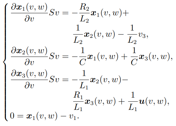
Problem 1 Find a dynamic control law u for the following system:

\{\begin{array}{l} {\dot{x}}_{1} = - \frac{R_{2}}{L_{2}} x_{1} + \frac{1}{L_{2}} x_{2} - \frac{1}{L_{2}} v_{3}, \\ {\dot{x}}_{2} = - \frac{1}{C} x_{1} + \frac{1}{C} x_{3}, \\ {\dot{x}}_{3} = - \frac{1}{L_{1}} x_{2} - \frac{R_{1}}{L_{1}} x_{3} + \frac{1}{L_{1}} u, \\ \dot{v} = S v, \\ e = y - v_{1}, \end{array}

(3)

that makes the controlled grid current y asymptotically tracks the given sinusoidal signal v₁ under the external sinusoidal disturbance v₃, i.e.,

\underset{t \to \infty}{l i m} e (t) = 0 .

3 Controller design and stability analysis

In this section, the paper will solve the controller design problem for grid-connected inverter, and solve the robust output regulation problem for the system (3) in a standard lower triangular form. To this end, the paper first establishes the elegant internal model to guarantee the asymptotic tracking under the unknown parameter uncertainty and disturbance.

As known from the output regulation framework, a necessary condition is that there exist zero-error constrained state and input, respectively, denoted by

(x_{1} (v, w), x_{2} (v, w), x_{3} (v, w))

and

u (v, w),

which satisfy the following regulator equations:

(4)

By calculation, the solution is obtained to regulator equations (4) as follows:

\{\begin{array}{l} x_{1} (v, w) = v_{1}, x_{2} (v, w) = R_{2} v_{1} + L_{2} σ v_{2} + v_{3}, \\ x_{3} (v, w) = (1 - L_{2} C σ^{2}) v_{1} + R_{2} C σ v_{2} + C σ v_{4}, \\ u (v, w) = a_{1} v_{1} + a_{2} v_{2} + a_{3} v_{3} + a_{4} v_{4}, \end{array}

(5)

where a₁ = R₁ (1 − L₂Cσ²) + R₂ (1 − L₁Cσ²) , a₂ = σ (L₁ −L₁L₂Cσ² +R₁R₂C +L₂) , a₃ = 1−L₁Cσ², and a₄ = R₁Cσ.

The solution provides the steady-state information

x_{i} (v, w), i = 1, 2, 3,

and

u (v, w)

when the grid-connected inverter achieves the tracking objective. However, due to the unavailable knowledge of v and w, it can not directly use the information for current tracker design. To solve this technical dilemma, the paper resorts to establish a dynamical compensator called internal model ^[21]. For simplicity, define

x_{4} (v, w) = u (v, w) .

Then, notice that

x_{i + 1} (v, w), i = 1, 2, 3,

are polynomial of v whose coefficients depend on w. In light of reference ^[21], it has

\{\begin{array}{l} \frac{\partial τ_{i} (v, w)}{\partial v} S v = Φ_{i} τ_{i} (v, w), \\ x_{i + 1} (v, w) = Γ_{i} τ_{i} (v, w), i = 1, 2, 3, \end{array}

(6)

where

τ_{i} (v, w) = [\begin{matrix} x_{i + 1} (v, w) \\ {\dot{x}}_{i + 1} (v, w) \end{matrix}], Φ_{i} = [\begin{matrix} 0 & 1 \\ - σ^{2} & 0 \end{matrix}], Γ_{i} = {[\begin{matrix} 1 \\ 0 \end{matrix}]}^{T} .

It can be observed that the pair

(Γ_{i}, Φ_{i})

is always observable. Choose Hurwitz matrix

M_{i} \in R^{2 \times 2}

and vector

N_{i} \in R^{2 \times 1}

for i = 1, 2, 3 such that the pair (M_i, N_i) is controllable. Since the spectra of M_i is disjoint from Φ_i, one can always obtain a nonsingular matrix T_i satisfying the Sylvester equation

T_{i} Φ_{i} - M_{i} T_{i} = N_{i} Γ_{i}

(7)

In this respect, denoting θ_i (v, w) = T_iτ_i (v, w) gives the steady-state generator

\begin{matrix} \frac{\partial θ_{i} (v, w)}{\partial v} S v = (M_{i} + N_{i} Ψ_{i}) θ_{i} (v, w), \\ x_{i + 1} (v, w) = Ψ_{i} θ_{i} (v, w), \end{matrix}

where

Ψ_{i} = Γ_{i} T_{i}^{- 1}

. Therefore, the internal model with outputxi+1 can be established as follows:

{\dot{η}}_{i} = M_{i} η_{i} + N_{i} x_{i + 1}, i = 1,2, 3

(8)

where x₄ = u.

The procedure of establishing the internal model (8) follows the general line in ^[21]. Technically, it provides the steady-state information for the tracking and disturbance rejection problem of inverter. As a result, perform the coordinate transformation defined as

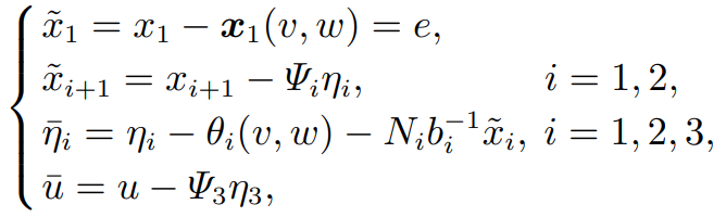
(9)

with

b_{1} = \frac{1}{L_{2}}, b_{2} = \frac{1}{C}

and

b_{3} = \frac{1}{L_{1}}

, it has the following system:

\{\begin{matrix} {\dot{\bar{η}}}_{i} = M_{i} {\bar{η}}_{i} + Θ_{i} ({\bar{η}}_{1}, \dots, {\bar{η}}_{i - 1}, {\tilde{x}}_{1}, \dots, {\tilde{x}}_{i}, w), \\ {\dot{\tilde{x}}}_{i} = Υ_{i} ({\bar{η}}_{1}, \dots, {\bar{η}}_{i}, {\tilde{x}}_{1}, \dots, {\tilde{x}}_{i}, w) + b_{i} {\tilde{x}}_{i + 1}, \end{matrix}

(10)

where

{\tilde{x}}_{4} = \bar{u}

and, for i = 1, 2, 3,

\begin{matrix} Θ_{i} ({\bar{η}}_{1}, \dots, {\bar{η}}_{i - 1}, {\tilde{x}}_{1}, \dots, {\tilde{x}}_{i}, w) = \\ M_{i} N_{i} b_{i}^{- 1} {\tilde{x}}_{i} - N_{i} b_{i}^{- 1} Δ_{i} ({\bar{η}}_{1}, \dots, {\bar{η}}_{i - 1}, {\tilde{x}}_{1}, \dots, {\tilde{x}}_{i}, w), \\ Υ_{i} ({\bar{η}}_{1}, \dots, {\bar{η}}_{i}, {\tilde{x}}_{1}, \dots, {\tilde{x}}_{i}, w) = \\ Δ_{i} ({\bar{η}}_{1}, \dots, {\bar{η}}_{i - 1}, {\tilde{x}}_{1}, \dots, {\tilde{x}}_{i}, w) + b_{i} Ψ_{i} ({\bar{η}}_{i} + N_{i} b_{i}^{- 1} {\tilde{x}}_{i}) . \end{matrix}

In the above equations, by merging and simplifying, it has

\begin{matrix} Δ_{1} (\cdot) = g_{11} {\tilde{x}}_{1}, Δ_{2} (\cdot) = h_{21} {\bar{η}}_{1} + g_{21} {\tilde{x}}_{1} + g_{22} {\tilde{x}}_{2}, \\ Δ_{3} (\cdot) = h_{31} {\bar{η}}_{1} + h_{32} {\bar{η}}_{2} + g_{31} {\tilde{x}}_{1} + g_{32} {\tilde{x}}_{2} + g_{33} {\tilde{x}}_{3}, \end{matrix}

with

\begin{matrix} g_{11} = - \frac{R_{2}}{L_{2}}, h_{21} = - Ψ_{1} (M_{1} + N_{1} Ψ_{1}), \\ g_{21} = - \frac{1}{C} - Ψ_{1} (M_{1} + N_{1} Ψ_{1}) N_{1} L_{2}, g_{22} = - Ψ_{1} N_{1}, \\ h_{31} = - \frac{1}{L_{1}} Ψ_{1}, h_{32} = - \frac{R_{1}}{L_{1}} Ψ_{2} - Ψ_{2} (M_{2} + N_{2} Ψ_{2}), \\ g_{31} = - \frac{1}{L_{1}} Ψ_{1} N_{1} L_{2}, g_{33} = - \frac{R_{1}}{L_{1}} - Ψ_{2} N_{2}, \\ g_{32} = - \frac{1}{L_{1}} - \frac{R_{1}}{L_{1}} Ψ_{2} N_{2} C - Ψ_{2} (M_{2} + N_{2} Ψ_{2}) N_{2} C . \end{matrix}

Notice that the transformed system (10) satisfies Θ_i (0, · · ·, 0, w) = 0 and Υ_i (0, · · ·, 0, w) = 0 for i = 1, 2, 3 and all

w \in W \subset R^{5} .

Therefore, the tracking control problem of system (3) has been turned to the robust stabilization problem of the transformed system (10) . Until now, it is ready to propose the following lemma.

Lemma 1 The robust stabilization control problem of the system (10) is solved by

\{\begin{array}{l} \bar{u} = - k_{3} {\bar{x}}_{3} \\ {\bar{x}}_{i + 1} = {\tilde{x}}_{i + 1} + k_{i} {\bar{x}}_{i}, i = 1, 2 \\ {\bar{x}}_{1} = {\tilde{x}}_{1} = e \end{array}

(11)

where k_i for i = 1, 2, 3, are positive constants to be determined.

The proof is provided in Appendix.

Remark 1 In the proof of Lemma1, k₁, k₂, k₃ need to be selected to satisfy

k_{1} ⩾ \frac{1}{2 b_{1}} (λ_{11} + 1), k_{2} ⩾ \frac{1}{2 b_{2}} (λ_{22} + 1)

and

k_{3} ⩾ \frac{1}{2 b_{3}} (λ_{33} + 1)

, respectively. In fact, it can also choose k₁, k₂, k₃ in another way, so that the closed-loop system is asymptotically stable. Let

\bar{x} = {[\begin{matrix} {\bar{x}}_{1} {\bar{x}}_{2} {\bar{x}}_{3} \end{matrix}]}^{T} \in R^{3}, \bar{η} = {[\begin{matrix} {\bar{η}}_{1}^{T} {\bar{η}}_{2}^{T} {\bar{η}}_{3}^{T} \end{matrix}]}^{T} \in R^{6},

and

{\bar{x}}_{c} = {[\begin{matrix} {\bar{x}}^{T} {\bar{η}}^{T} \end{matrix}]}^{T} .

Thus, it has the following system:

\{\begin{matrix} \dot{\bar{x}} = A_{1} \bar{x} + B_{1} \bar{η}, \\ \dot{\bar{η}} = A_{2} \bar{x} + B_{2} \bar{η}, \end{matrix}

(12)

where

\begin{matrix} A_{1} = [\begin{matrix} φ_{11} - b_{1} k_{1} & b_{1} & 0 \\ φ_{21} & φ_{22} - b_{2} k_{2} & b_{2} \\ φ_{31} & φ_{32} & φ_{33} - b_{3} k_{3} \end{matrix}], \\ B_{1} = [\begin{matrix} ϕ_{11} & 0 & 0 \\ ϕ_{21} & ϕ_{22} & 0 \\ ϕ_{31} & ϕ_{32} & ϕ_{33} \end{matrix}], \\ A_{2} = [\begin{matrix} f_{11} & 0 & 0 \\ f_{21} & f_{22} & 0 \\ f_{31} & f_{32} & f_{33} \end{matrix}], B_{2} = [\begin{matrix} M_{1} & 0 & 0 \\ l_{21} & M_{2} & 0 \\ l_{31} & l_{32} & M_{3} \end{matrix}] . \end{matrix}

It further has

{\dot{\bar{x}}}_{c} = [\begin{matrix} A_{1} B_{1} \\ A_{2} B_{2} \end{matrix}] {\bar{x}}_{c} ≜ A_{c} {\bar{x}}_{c}

(13)

If we can choose k₁, k₂ and k₃such that the matrix A_c is Hurwitz, then the system (13) is asymptotically stable. In addition, the transient response index of the system can be guaranteed by adjusting parameter k₁, k₂ and k₃.

Further, it has the main results as follows.

Theorem 1 Problem 1 is solved by the following dynamic controller

\{\begin{array}{l} u = - k_{3} {\bar{x}}_{3} + Ψ_{3} η_{3}, \\ {\dot{η}}_{i} = M_{i} η_{i} + N_{i} x_{i + 1}, i = 1, 2, 3, \\ {\bar{x}}_{1} = e, \\ {\bar{x}}_{i + 1} = x_{i + 1} - Ψ_{i} η_{i} + k_{i} {\bar{x}}_{i}, i = 1, 2 . \end{array}

(14)

The proof is provided in Appendix.

4 Simulation verification

In this subsection, the simulation tests on a threephase grid-connected inverter are conducted to illustrate the efficiency of the proposed feedback control scheme and the comparison with the feedforward control method is shown to reinforce this effect by using MATLAB/Simulink platform.

The range of system parameters used in the simulation are listed in Table1. A sine current configured with A_r = 10 A, ϕ_r = 0 rad is taken as the desired output current injected into the grid and a sine voltage with

A_{d} = 220 \sqrt{2} V, ϕ_{d} = \frac{π}{3}

rad is chosen as the interfacing disturbance voltage, for which the nominal values R₁ = 1.8 Ω, L₁ = 600 µH, R₂ = 1.4 Ω, L₂ = 700 µH and C = 15 µF (represented by Case1) and the uncertain parameters R₁ = 2.5 Ω, L₁ = 450 µH, R₂ = 0.8 Ω, L₂ = 450 µH, C = 12 µF (represented by Case2) are used in LCL-filter to produce the actual output current I_O (t) and to verify the robustness performance against parameter uncertainty.

Table1System parameters

As shown in Table1, the power frequency f = 50 Hz, then it has σ = 100π and

S = [\begin{matrix} 0 & 100 π & 0 & 0 \\ - 100 π & 0 & 0 & 0 \\ 0 & 0 & 0 & 100 π \\ 0 & 0 & - 100 π & 0 \end{matrix}]

It further has y_r (t) = v₁ (t) = 10 sin (100πt) and

V_{G} (t) = v_{3} (t) = 220 \sqrt{2} s i n (100 π t + \frac{π}{6})

According to Eq. (6) , for i = 1, 2, 3, it has

Φ_{i} = [\begin{matrix} 0 & 1 \\ - 10000 π^{2} & 0 \end{matrix}], Γ_{i} = [\begin{matrix} 1 0 \end{matrix}] .

Choose the controllable pair (M_i, N_i) for i = 1, 2, 3 as

M_{1} = [\begin{matrix} 0 & 1 \\ - 2600 & - 1200 \end{matrix}], N_{1} = [\begin{matrix} 0 \\ 1 \end{matrix}],

\begin{matrix} M_{2} = [\begin{matrix} 0 & 1 \\ - 2500 & - 1200 \end{matrix}], N_{2} = [\begin{matrix} 0 \\ 1 \end{matrix}], \\ M_{3} = [\begin{matrix} 0 & 1 \\ - 1200 & - 1000 \end{matrix}], N_{3} = [\begin{matrix} 0 \\ 1 \end{matrix}] . \end{matrix}

By the solution T_i, i = 1, 2, 3 of the Sylvester equation (7) , it further has

\begin{matrix} Ψ_{1} = Γ_{1} T_{1}^{- 1} = [\begin{matrix} - 9.6096 \times 10^{4} & 1.2000 \times 10^{3} \end{matrix}], \\ Ψ_{2} = Γ_{2} T_{2}^{- 1} = [\begin{matrix} - 9.6196 \times 10^{4} & 1.2000 \times 10^{3} \end{matrix}], \\ Ψ_{3} = Γ_{3} T_{3}^{- 1} = [\begin{matrix} - 9.7496 \times 10^{4} & 1.2000 \times 10^{3} \end{matrix}] . \end{matrix}

Then, by Theorem 1, a dynamic state feedback controller (14) is designed with k₁ = 12, k₂ = 0.035, k₃ = 340.

Since the input voltage VI of each phase for a threephase grid-connected inverter cannot be controlled directly, it needs to use the input signal u as modulation signal to generate the gate drive signals by space vector pulse width modulation (SVPWM) technique. Then, the inverter is driven by the gate drive signals and generates the driving voltage for each phase. Under the supervisory of the developed feedback controller, the grid-connected inverter can form the required reference voltage after the transient fluctuation of its output voltage. The simulation model and the controller model are shown in Fig.2 and Fig.3, respectively.

Similarly, the paper sets two groups of system parameters like the nominal values and the uncertain parameters to observe the tracking performance of the output current and verify the robustness of our controller, and present the results in Fig.4 and Fig.5. It should be noted that e_A, e_B, e_C represent the current tracking error for phase A, phase B and phase C, respectively.

Fig.2Simulation model for the proposed control scheme

Fig.3The proposed controller of block diagram

Fig.4Tracking errors under the proposed controller (14)

Fig.4 shows the output current tracking errors e = I_O − y_r with the nominal and uncertain grid-connected inverter values, respectively, and the results show that the output current signal I_O can quickly follow the reference current signal y_r under the proposed controlscheme. Fig.5 shows the corresponding total harmonic distortion (THD) analysis of output current I_O of phase A in the above two test conditions. The THD values are 0.85% and 1.14% (<5%) , respectively, which indicates that the output current meets the requirements. The same conclusion holds for currents of other phases. Therefore, under the internal model based feedback controller (14) , the tracking performance can be maintained despite the changes in the system parameters, which validates the robustness of the proposed controller (14) .

Fig.5THD analysis under the proposed controller (14)

To better demonstrate the performance of the proposed control strategy, the paper uses a feedforward control method based on regulator equations for comparison. For the grid-connected inverter with nominal system parameters, under the assumption that the system states in Eq. (3) and the exosystem signals in Eq. (2) can be available, the feedforward control law can then be directly employed.

By Eq. (3) , it has the following system

\{\begin{array}{l} \dot{x} = A_{3} x + B_{3} u + E_{3} v, \\ e = C_{3} x + F_{3} v, \\ \dot{v} = S v, \end{array}

(15)

where

x = {[\begin{matrix} x_{1} x_{2} x_{3} \end{matrix}]}^{T} \in R^{3}

and

\begin{matrix} A_{3} = [\begin{matrix} - \frac{R_{2}}{L_{2}} & \frac{1}{L_{2}} & 0 \\ - \frac{1}{C} & 0 & \frac{1}{C} \\ 0 & - \frac{1}{L_{1}} & - \frac{R_{1}}{L_{1}} \end{matrix}], B_{3} = [\begin{matrix} 0 \\ 0 \\ \frac{1}{L_{1}} \end{matrix}], \\ E_{3} = [\begin{matrix} 0 & 0 & - \frac{1}{L_{2}} & 0 \\ 0 & 0 & 0 & 0 \\ 0 & 0 & 0 & 0 \end{matrix}], C_{3} = [\begin{matrix} 1 & 0 & 0 \end{matrix}], \\ F_{3} = [\begin{matrix} - 1 & 0 & 0 & 0 \end{matrix}] . \end{matrix}

It’s easy to prove that all the eigenvalues of S have no negative real parts, and the pair (A₃, B₃) is controllable. Furthermore, the regulator equations

\{\begin{array}{l} X S = A_{3} X + B_{3} U + E_{3}, \\ 0 = C_{3} X + F_{3}, \end{array}

(16)

have a solution (X, U) with

X = [\begin{matrix} X_{11} X_{12} X_{13} X_{14} \\ X_{21} X_{22} X_{23} X_{24} \\ X_{31} X_{32} X_{33} X_{34} \end{matrix}], U = [\begin{matrix} U_{1} U_{2} U_{3} U_{4} \end{matrix}],

where

\begin{matrix} X_{11} = 1, X_{12} = 0, X_{13} = 0, X_{14} = 0, X_{21} = R_{2}, \\ X_{22} = L_{2} σ, X_{23} = 1, X_{24} = 0, X_{31} = 1 - L_{2} C σ^{2}, \\ X_{32} = R_{2} C σ, X_{33} = 0, X_{34} = C σ, \\ U_{1} = - (R_{1} L_{2} + R_{2} L_{1}) C σ^{2} + R_{2} + R_{1}, \\ U_{2} = L_{1} (1 - L_{2} C σ^{2}) σ + (L_{2} + R_{1} R_{2} C) σ, \\ U_{3} = 1 - L_{1} C σ^{2}, U_{4} = R_{1} C σ . \end{matrix}

Therefore, by ^[22], it can design a feedforward controller as follows:

u = K_{1} x + K_{2} v,

(17)

where K₁ makes the matrix A₃ +B₃K₁ is Hurwitz and K₂ = U−K₁X. Here, the expected eigenvalues of matrix A₃+B₃K₁ are equipped with {−20 300, −20 800, −20 400}, then it obtains K₁ = [−5.381 1 − 8.418 0 −33.900 0] and K₂ = [54.228 0 2.494 9 9.417 1 0.168 2].

With the same parameter conditions and SVPWM mechanism, a simulation under the feedforward controller (17) is performed as a comparison with our controller (14) , and its results are given in Fig.6 and Fig.7. In Fig.6 and Fig.7, one can see that the output current tracking errors can converge to the neighborhood of the origin under the nominal parameter condition, but not under the uncertain parameter condition, which indicates that, in contrast to the proposed control strategy (14) , the feedforward controller (17) cannot tolerate the parameter uncertainty.

Fig.6Tracking errors under the feedforward controller (17)

As a result, our controller (14) has more advantages in maintaining the system performance and suppressing the variation of system parameter. In other words, the proposed controller is robust, while the feedforward controller is not.

In MATLAB/Simulink experiments, due to the influence of SVPWM and the existence of harmonic com-ponents, the current tracking error is not asymptotically stable under the proposed control strategy. However, from Fig.4–7, the comparison with the feedforward controller still shows that our controller (14) has better robustness to suppress the parameter uncertainty.

Fig.7THD analysis under the feedforward controller (17)

5 Conclusions

This article has researched the robust current tracking control problem of the three-phase grid-connected inverters with external sinusoidal disturbances. By the internal model principle, a solution to the problem has been presented by a dynamic state feedback control law. Furthermore, the parameter uncertainty and the grid voltage disturbance have been well handled and the performance recovery has been achieved under the proposed control strategy. In the future, the research will consider an output-based control strategy and extend the results to micro-grid experiment platforms.

Appendix Proof of Lemma 1

Proof Choose

V_{i}^{1} = {\bar{l}}_{i} {\bar{η}}_{i}^{T} P_{i} {\bar{η}}_{i},

where

{\bar{l}}_{i}

for i = 1, 2, 3, are positive constants to be specified later, P_i satisfying the following Lyapunov equation:

P_{i} M_{i} + M_{i}^{T} P_{i} = - I .

Similar to Eq. (11) , let

{\bar{x}}_{1} = {\tilde{x}}_{1}, {\bar{x}}_{i + 1} = {\tilde{x}}_{i + 1} + k_{i} {\bar{x}}_{i}, i = 1, 2, 3,

with

{\bar{x}}_{4} = 0

and k_ibeing some positive constants to be specified later.

For the first subsystem

({\bar{η}}_{1}, {\bar{x}}_{1})

of Eq. (10) , it has

\begin{matrix} {\dot{\bar{η}}}_{1} = M_{1} {\bar{η}}_{1} + f_{11} {\bar{x}}_{1}, \\ {\dot{\bar{x}}}_{1} = ϕ_{11} {\bar{η}}_{1} + φ_{11} {\bar{x}}_{1} + b_{1} ({\bar{x}}_{2} - k_{1} {\bar{x}}_{1}), \end{matrix}

where

f_{11} = M_{1} N_{1} b_{1}^{- 1} - N_{1} b_{1}^{- 1} g_{11}, ϕ_{11} = b_{1} Ψ_{1}, φ_{11} = Ψ_{1} N_{1} + g_{11} .

Letting

V_{1} = {\bar{l}}_{1} {\bar{η}}_{1}^{T} P_{1} {\bar{η}}_{1} + {\bar{x}}_{1}^{2}

gives

\begin{matrix} {\dot{V}}_{1} = {\bar{l}}_{1} (- {‖{\bar{η}}_{1}‖}^{2} + 2 {\bar{η}}_{1}^{T} P_{1} f_{11} {\bar{x}}_{1}) + 2 {\bar{x}}_{1} (ϕ_{11} {\bar{η}}_{1} + \\ φ_{11} {\bar{x}}_{1} + b_{1} {\bar{x}}_{2}) - 2 b_{1} k_{1} {\bar{x}}_{1}^{2} ⩽ \\ {\bar{l}}_{1} (- {‖{\bar{η}}_{1}‖}^{2} + ϵ_{1} ‖P_{1} f_{11}‖ {‖{\bar{η}}_{1}‖}^{2} + ϵ_{1}^{- 1} ‖P_{1} f_{11}‖ {\bar{x}}_{1}^{2}) + \\ ‖ϕ_{11}‖ {‖{\bar{η}}_{1}‖}^{2} + ‖ϕ_{11}‖ {\bar{x}}_{1}^{2} + 2 φ_{11} {\bar{x}}_{1}^{2} + b_{1} {\bar{x}}_{1}^{2} + \\ b_{1} {\bar{x}}_{2}^{2} - 2 b_{1} k_{1} {\bar{x}}_{1}^{2} ⩽ \\ - ρ_{11} {‖{\bar{η}}_{1}‖}^{2} + (λ_{11} - 2 b_{1} k_{1}) {\bar{x}}_{1}^{2} + b_{1} {\bar{x}}_{2}^{2}, \end{matrix}

where

\begin{matrix} ρ_{11} = {\bar{l}}_{1} (1 - ϵ_{1} ‖P_{1} f_{11}‖) - ‖ϕ_{11}‖ \\ λ_{11} = {\bar{l}}_{1} ϵ_{1}^{- 1} ‖P_{1} f_{11}‖ + ‖ϕ_{11}‖ + 2 φ_{11} + b_{1} . \end{matrix}

It can be concluded that there exists positive constants

{\bar{l}}_{1}

and

ϵ_{1}

yielding

ρ_{11} ⩾ 1 .

Choosing k₁ >

\frac{1}{2 b_{1}} (λ_{11} + 1),

it has

{\dot{V}}_{1} ⩽ - {‖{\bar{η}}_{1}‖}^{2} - {\bar{x}}_{1}^{2} + b_{1} {\bar{x}}_{2}^{2} .

(A1)

For the second subsystem

({\bar{η}}_{2}, {\bar{x}}_{2}),

it follows that

\begin{matrix} {\dot{\bar{η}}}_{2} = M_{2} {\bar{η}}_{2} + l_{21} {\bar{η}}_{1} + f_{21} {\bar{x}}_{1} + f_{22} {\bar{x}}_{2}, \\ {\dot{\bar{x}}}_{2} = ϕ_{21} {\bar{η}}_{1} + ϕ_{22} {\bar{η}}_{2} + φ_{21} {\bar{x}}_{1} + φ_{22} {\bar{x}}_{2} + b_{2} ({\bar{x}}_{3} - k_{2} {\bar{x}}_{2}), \end{matrix}

where

\begin{matrix} l_{21} = - N_{2} b_{2}^{- 1} h_{21} \\ f_{21} = - M_{2} N_{2} b_{2}^{- 1} k_{1} - N_{2} b_{2}^{- 1} g_{21} + N_{2} b_{2}^{- 1} g_{22} k_{1} \\ f_{22} = M_{2} N_{2} b_{2}^{- 1} - N_{2} b_{2}^{- 1} g_{22} \\ ϕ_{21} = h_{21} + k_{1} ϕ_{11}, ϕ_{22} = b_{2} Ψ_{2} \\ φ_{21} = g_{21} - φ_{22} k_{1} + φ_{11} k_{1}, φ_{22} = g_{22} + Ψ_{2} N_{2} + b_{1} k_{1} . \end{matrix}

Defining

V_{2} = p_{1} V_{1} + {\bar{l}}_{2} {\bar{η}}_{2}^{T} P_{2} {\bar{η}}_{2} + {\bar{x}}_{2}^{2}

leads to

\begin{matrix} {\dot{V}}_{2} = p_{1} {\dot{V}}_{1} + {\bar{l}}_{2} (- {‖{\bar{η}}_{2}‖}^{2} + 2 {\bar{η}}_{2}^{T} P_{2} l_{21} {\bar{η}}_{1} + \\ 2 {\bar{η}}_{2}^{T} P_{2} f_{21} {\bar{x}}_{1} + 2 {\bar{η}}_{2}^{T} P_{2} f_{22} {\bar{x}}_{2}) + \\ 2 {\bar{x}}_{2} (ϕ_{21} {\bar{η}}_{1} + ϕ_{22} {\bar{η}}_{2} + φ_{21} {\bar{x}}_{1} + \\ φ_{22} {\bar{x}}_{2} + b_{2} {\bar{x}}_{3}) - 2 b_{2} k_{2} {\bar{x}}_{2}^{2} ⩽ \\ - (p_{1} - {\bar{l}}_{2} ϵ_{2}^{- 1} ‖P_{2} l_{21}‖ - ‖ϕ_{21}‖) {‖{\bar{η}}_{1}‖}^{2} - \\ ({\bar{l}}_{2} (1 - ϵ_{2} ‖P_{2} l_{21}‖ - ϵ_{2} ‖P_{2} f_{21}‖ - ϵ_{2} ‖P_{2} f_{22}‖) - \\ ‖ϕ_{22}‖) {‖{\bar{η}}_{2}‖}^{2} - (p_{1} - {\bar{l}}_{2} ϵ_{2}^{- 1} ‖P_{2} f_{21}‖ - ‖φ_{21}‖) {\bar{x}}_{1}^{2} + \\ (p_{1} b_{1} + {\bar{l}}_{2} ϵ_{2}^{- 1} ‖P_{2} f_{22}‖ + ‖ϕ_{21}‖ + ‖ϕ_{22}‖ + \\ ‖φ_{21}‖ + 2 φ_{22} + b_{2} - 2 b_{2} k_{2}) {\bar{x}}_{2}^{2} + b_{2} {\bar{x}}_{3}^{2} = \\ - ρ_{21} {‖{\bar{η}}_{1}‖}^{2} - ρ_{22} {‖{\bar{η}}_{2}‖}^{2} - λ_{21} {\bar{x}}_{1}^{2} + (λ_{22} - \\ 2 b_{2} k_{2}) {\bar{x}}_{2}^{2} + b_{2} {\bar{x}}_{3}^{2}, \end{matrix}

where

\begin{matrix} ρ_{21} = p_{1} - {\bar{l}}_{2} ϵ_{2}^{- 1} ‖P_{2} l_{21}‖ - ‖ϕ_{21}‖, \\ ρ_{22} = {\bar{l}}_{2} (1 - ϵ_{2} ‖P_{2} l_{21}‖ - ϵ_{2} ‖P_{2} f_{21}‖ - \\ ϵ_{2} ‖P_{2} f_{22}‖) - ‖ϕ_{22}‖, \\ λ_{21} = p_{1} - {\bar{l}}_{2} ϵ_{2}^{- 1} ‖P_{2} f_{21}‖ - ‖φ_{21}‖, \\ λ_{22} = p_{1} b_{1} + {\bar{l}}_{2} ϵ_{2}^{- 1} ‖P_{2} f_{22}‖ + ‖ϕ_{21}‖ + \\ ‖ϕ_{22}‖ + ‖φ_{21}‖ + 2 φ_{22} + b_{2} . \end{matrix}

Choose

{\bar{l}}_{2}

and

ϵ_{2}

such that

ρ_{22} ⩾ 1 .

Then, one can always find a positive constant p₁ assuring ρ₂₁ ≥ 1 and λ₂₁ ≥1. Letting

k_{2} ⩾ \frac{1}{2 b_{2}} (λ_{22} + 1)

gives

{\dot{V}}_{2} ⩽ - {‖{\bar{η}}_{1}‖}^{2} - {‖{\bar{η}}_{2}‖}^{2} - {\bar{x}}_{1}^{2} - {\bar{x}}_{2}^{2} + b_{2} {\bar{x}}_{3}^{2} .

(A2)

Moreover, the third subsystem

({\bar{η}}_{3}, {\bar{x}}_{3})

can be rewritten as

\begin{matrix} {\dot{\bar{η}}}_{3} = M_{3} {\bar{η}}_{3} + l_{31} {\bar{η}}_{1} + l_{32} {\bar{η}}_{2} + f_{31} {\bar{x}}_{1} + f_{32} {\bar{x}}_{2} + f_{33} {\bar{x}}_{3}, \\ {\dot{\bar{x}}}_{3} = ϕ_{31} {\bar{η}}_{1} + ϕ_{32} {\bar{η}}_{2} + ϕ_{33} {\bar{η}}_{3} + φ_{31} {\bar{x}}_{1} + φ_{32} {\bar{x}}_{2} + \end{matrix}

φ_{33} {\bar{x}}_{3} + b_{3} (- k_{3} {\bar{x}}_{3}),

where

\begin{matrix} l_{31} = - N_{3} b_{3}^{- 1} h_{31}, l_{32} = - N_{3} b_{3}^{- 1} h_{32}, \\ f_{31} = - N_{3} b_{3}^{- 1} g_{31} + N_{3} b_{3}^{- 1} g_{32} k_{1}, \\ f_{32} = - M_{3} N_{3} b_{3}^{- 1} k_{2} - N_{3} b_{3}^{- 1} g_{32} + N_{3} b_{3}^{- 1} g_{33} k_{2}, \\ f_{33} = M_{3} N_{3} b_{3}^{- 1} - N_{3} b_{3}^{- 1} g_{33}, \\ ϕ_{31} = h_{31} + k_{2} ϕ_{21}, \\ ϕ_{32} = h_{32} + k_{2} ϕ_{22}, ϕ_{33} = b_{3} Ψ_{3}, \\ φ_{31} = g_{31} - g_{32} k_{1} + φ_{21} k_{2}, \\ φ_{32} = g_{32} - φ_{33} k_{2} + φ_{22} k_{2}, \\ φ_{33} = g_{33} + Ψ_{3} N_{3} + b_{2} k_{2} . \end{matrix}

Defining

V_{3} = p_{2} V_{2} + {\bar{l}}_{3} {\bar{η}}_{3}^{T} P_{3} {\bar{η}}_{3} + {\bar{x}}_{3}^{2},

one can obtain

\begin{matrix} {\dot{V}}_{3} = p_{2} {\dot{V}}_{2} + {\bar{l}}_{3} (- {‖{\bar{η}}_{3}‖}^{2} + 2 {\bar{η}}_{3}^{T} P_{3} l_{31} {\bar{η}}_{1} + \\ 2 {\bar{η}}_{3}^{T} P_{3} l_{32} {\bar{η}}_{2} + 2 {\bar{η}}_{3}^{T} P_{3} f_{31} {\bar{x}}_{1} + 2 {\bar{η}}_{3}^{T} P_{3} f_{32} {\bar{x}}_{2} + \\ 2 {\bar{η}}_{3}^{T} P_{3} f_{33} {\bar{x}}_{3}) + 2 {\bar{x}}_{3} (ϕ_{31} {\bar{η}}_{1} + ϕ_{32} {\bar{η}}_{2} + ϕ_{33} {\bar{η}}_{3} + \\ φ_{31} {\bar{x}}_{1} + φ_{32} {\bar{x}}_{2} + φ_{33} {\bar{x}}_{3} + b_{3} (- k_{3} {\bar{x}}_{3})) ⩽ \\ - (p_{2} - {\bar{l}}_{3} ϵ_{3}^{- 1} ‖P_{3} l_{31}‖ - ‖ϕ_{31}‖) {‖{\bar{η}}_{1}‖}^{2} - \\ (p_{2} - {\bar{l}}_{3} ϵ_{3}^{- 1} ‖P_{3} l_{32}‖ - ‖ϕ_{32}‖) {‖{\bar{η}}_{2}‖}^{2} - \\ ({\bar{l}}_{3} (1 - ϵ_{3} ‖P_{3} l_{31}‖ - ϵ_{3} ‖P_{3} l_{32}‖ - ϵ_{3} ‖P_{3} f_{31}‖ - \\ ϵ_{3} ‖P_{3} f_{32}‖ - ϵ_{3} ‖P_{3} f_{33}‖) - ‖ϕ_{33}‖) {‖{\bar{η}}_{3}‖}^{2} - \\ (p_{2} - {\bar{l}}_{3} ϵ_{3}^{- 1} ‖P_{3} f_{31}‖ - ‖φ_{31}‖) {\bar{x}}_{1}^{2} - \\ (p_{2} - {\bar{l}}_{3} ϵ_{3}^{- 1} ‖P_{3} f_{32}‖ - ‖φ_{32}‖) {\bar{x}}_{2}^{2} + \\ (p_{2} b_{2} + {\bar{l}}_{3} ϵ_{3}^{- 1} ‖P_{3} f_{33}‖ + ‖ϕ_{31}‖ + ‖ϕ_{32}‖ + \\ ‖ϕ_{33}‖ + ‖φ_{31}‖ + ‖φ_{32}‖ + 2 φ_{33} - 2 b_{3} k_{3}) {\bar{x}}_{3}^{2} = \\ - ρ_{31} {‖{\bar{η}}_{1}‖}^{2} - ρ_{32} {‖{\bar{η}}_{2}‖}^{2} - ρ_{33} {‖{\bar{η}}_{3}‖}^{2} - λ_{31} {\bar{x}}_{1}^{2} - \\ λ_{32} {\bar{x}}_{2}^{2} + (λ_{33} - 2 b_{3} k_{3}) {\bar{x}}_{3}^{2}, \end{matrix}

where

\begin{matrix} ρ_{31} = p_{2} - {\bar{l}}_{3} ϵ_{3}^{- 1} ‖P_{3} l_{31}‖ - ‖ϕ_{31}‖, \\ ρ_{32} = p_{2} - {\bar{l}}_{3} ϵ_{3}^{- 1} ‖P_{3} l_{32}‖ - ‖ϕ_{32}‖, \\ ρ_{33} = {\bar{l}}_{3} (1 - ϵ_{3} ‖P_{3} l_{31}‖ - ϵ_{3} ‖P_{3} l_{32}‖ - ϵ_{3} ‖P_{3} f_{31}‖ - \\ ϵ_{3} ‖P_{3} f_{32}‖ - ϵ_{3} ‖P_{3} f_{33}‖) - ‖ϕ_{33}‖, \\ λ_{31} = p_{2} - {\bar{l}}_{3} ϵ_{3}^{- 1} ‖P_{3} f_{31}‖ - ‖φ_{31}‖, \\ λ_{32} = p_{2} - {\bar{l}}_{3} ϵ_{3}^{- 1} ‖P_{3} f_{32}‖ - ‖φ_{32}‖, \\ λ_{33} = p_{2} b_{2} + {\bar{l}}_{3} ϵ_{3}^{- 1} ‖P_{3} f_{33}‖ + ‖ϕ_{31}‖ + \\ ‖ϕ_{32}‖ + ‖ϕ_{33}‖ + ‖φ_{31}‖ + ‖φ_{32}‖ + 2 φ_{33} . \end{matrix}

One can choose positive constants

{\bar{l}}_{3}

and

ϵ_{3}

such that ρ₃₃ ≥ 1 is satisfied. In addition, there always exists a positive constant p₂ satisfying ρ₃₁ ≥ 1, ρ₃₂ ≥ 1, λ₃₁ ≥ 1, λ₃₂ ≥ 1. Letting

k_{3} ⩾ \frac{1}{2 b_{3}} (λ_{33} + 1),

it obtains

{\dot{V}}_{3} ⩽ - {‖{\bar{η}}_{1}‖}^{2} - {‖{\bar{η}}_{2}‖}^{2} - {‖{\bar{η}}_{3}‖}^{2} - {\bar{x}}_{1}^{2} - {\bar{x}}_{2}^{2} - {\bar{x}}_{3}^{2} .

(A3)

Since V₃ is a positive definite function satisfying (A3) , it can conclude that

{\bar{η}}_{i}

and

{\bar{x}}_{i}, i = 1, 2, 3,

are bounded for all t ≥ 0 and square integrable on [0, ∞) . Using Barbalat’s lemma,

{\bar{η}}_{i}

and

{\bar{x}}_{i}, i = 1, 2, 3,

approach zero as t → ∞, and therefore, the closed-loop system is asymptotically stable for w ranging over a compact set W.

Proof of Theorem 1

Proof First, based on Lemma1 and for all t ≥ 0, we obtain that

{\bar{x}}_{i}, {\bar{η}}_{i}, i = 1, 2, 3,

are bounded. Also, it is known that v and w are bounded. Then, according to the transformation (9) , it can conclude that

x_{i}, η_{i}, i = 1, 2, 3,

and u are bounded. That is to say, all trajectories of the whole closed-loop system formed by Eq. (3) and Eq. (14) is bounded.

Second, based on Lemma1, the system (12) is asymptotically stable. Thus, it has

\underset{t \to \infty}{l i m} {\bar{x}}_{c} (t) = 0,

which together with the definitionof

{\bar{x}}_{c}

leads to

\underset{t \to \infty}{l i m} e (t) = 0 .

As a result, Problem 1 has been solved.

引用本文

刘伟, 吴本, 孙伟杰, 等. 带LCL滤波器的三相并网逆变器的鲁棒电流跟踪控制. 控制理论与应用, 2026, 43(1): 41 – 51

复制

LIU Wei, WU Ben, SUN Weijie, et al. Robust current tracking control for three-phase grid-connected inverters with LCL filter. Control Theory & Applications, 2026, 43(1): 41 – 51

Copy

计量

LIN X, LIU Y, YU J,et al. Stability analysis of three-phase gridconnected inverter under the weak grids with asymmetrical grid impedance by LTP theory in time domain. International Journal of Electrical Power & Energy Systems,2022,142:108244.

WANG B, XU Y, SHEN Z,et al. Current control of grid-connected inverter with LCL filter based on extended-state observer estimations using single sensor and achieving improved robust observation dynamics. IEEE Transactions on Industrial Electronics,2017,64(7):5428-5439.

HE J, LI Y W. Generalized closed-loop control schemes with embedded virtual impedances for voltage source converters with LC or LCL filters. IEEE Transactions on Power Electronics,2012,27(4):1850-1861.

SOLATIALKARAN D, ZARE F, SAHA T K,et al. A novel approach in filter design for grid-connected inverters used in renewable energy systems. IEEE Transactions on Sustainable Energy,2020,11(1):154-164.

CAI Y, HE Y, ZHOU H,et al. Design method of LCL filter for gridconnected inverter based on particle swarm optimization and screening method. IEEE Transactions on Power Electronics,2021,36(9):10097-10113.

VAMVOUDAKIS K G, POUR S F R, HESPANHA J P. Robust eventtriggered output feed-back learning algorithm for voltage source inverters with unknown load and parameter variations. International Journal of Robust and Nonlinear Control,2019,29:3502-3517.

MA G, XIE C, LI C,et al. Passivity-based design of external passive damper for LCL-type grid-connected inverter. IEEE Transactions on Power Electronics,2024,39(9):11558-11570.

ERROUISSI R, Al-DURRA A. Design of PI controller together with active damping for grid-tied LCL-filter systems using disturbanceobserver-based control approach. IEEE Transactions on Industry Applications,2018,54(4):3820-3831.

YU J, LIN X, SONG D,et al. New perspectives on stability analysis of three-phase grid-connected inverter considering system couplings. IEEE Transactions on Power Systems,2020,35(3):1967-1978.

TWINING E, HOLMES D. Grid current regulation of a three-phase voltage source inverter with an LCL input filter. IEEE Transactions on Power Electronics,2003,18(3):888-895.

KUPERMAN A. Proportional-resonant current controllers design based on desired transient performance. IEEE Transactions on Power Electronics,2015,30(10):5341-5345.

RODRIGUEZ J, KAZMIERKOWSKI M P, ESPINOZA J R,et al. State of the art of finite control set model predictive control in power electronics. IEEE Transactions on Industrial Informatics,2013,9(2):1003-1016.

TOSO F, FAVATO A, TORCHIO R,et al. Continuous control set model predictive current control of a microgrid-connected PWM inverter. IEEE Transactions on Power Systems,2021,36(1):415-425.

NAM N N, NGUYEN N D, YOON C,et al. Voltage sensorless model predictive control for a grid-connected inverter with LCL filter. IEEE Transactions on Industrial Electronics,2022,69(1):740-751.

YANG Bo, THIDAR Swe, ZHONG Lin’en,et al. Robust fractionalorder sliding-mode control design of grid-connected photovoltaic inverters. Control Theory & Applications,2020,37(2):374-386.(杨博, THIDAR Swe, 钟林恩, 等. 并网光伏逆变器鲁棒分数阶滑模控制设. 控制理论与应用,2020,37(2):374-386.)

PHD B L, LU P, ZHAN D,et al. Adaptive fuzzy fractional-order sliding-mode control of LCLinterfaced grid-connected converter with reduced-order. ISA Transactions,2023,132:557-572.

ZHENG Xuemei, SHI Xu, CHEN Xin,et al. Research on finite-time full-order sliding mode control of self-synchronous grid-connected inverter. Control Theory & Applications,2023,40(11):1903-1910.(郑雪梅, 时旭, 陈鑫, 等. 自同步型并网逆变器有限时间全阶终端滑模控制研究. 控制理论与应用,2023,40(11):1903-1910.)

KOCH G G, MACCARI L A, OLIVEIRA R C L F,et al. Robust H∞ state feedback controllers based on linear matrix inequalities applied to grid-connected converters. IEEE Transactions on Industrial Electronics,2019,66(8):6021-6031.

BELOV A. Robust pole placement and random disturbance rejection for linear polytopic systems with application to grid-connected converters. European Journal of Control,2022,63:116-125.

HUANG M, DING L, LI W,et al. Distributed observer-based H∞ fault-tolerant control for DC microgrids with sensor fault. IEEE Transactions on Circuits and Systems I: Regular Papers,2021,68(4):1659-1670.

HUANG J, CHEN Z. A general framework for tackling the output regulation problem. IEEE Transactions on Automatic Control,2004,49(12):2203-2218.

HUANG J. Nonlinear Output Regulation: Theory and Applications. Philadelphia, PA: SIAM,2004.

ERROUISSI R, Al-DURRA A. A novel control technique for gridtied inverters considering unbalanced grid voltage conditions and control input saturation. IEEE Transactions on Sustainable Energy,2019,10(4):2223-2234.

ERROUISSI R, SHAREEF H, AWWAD F. Disturbance observerbased control for three-phase grid-tied inverter with LCL filter. IEEE Transactions on Industry Applications,2021,57(5):5411-5424.

AHMED K H, MASSOUD A M, FINNEY S J,et al. A modified stationary reference frame-based predictive current control with zero steady-state error for LCL coupled inverter-based distributed generation systems. IEEE Transactions on Industrial Electronics,2011,58(4):1359-1370.